Covid 19 Model
Numerical simulations and applications of the model developed my pulication with M. S. Aronna and R. Guglielmi
Numerical simulations and applications of the model described in the publication entitled A model for COVID-19 with isolation, quarantine and testing as control measures, a publication that I was co-author.
In addition to the model description, the article shows numerical simulations to check the model and make some appointments about the disease, in special about the non-pharmaceutical control measures such as isolation, quarantine and testing. The model and the simulations were written in Python language.
In the README, it’s possible to understand how to use the model after changing the desired parameters. In order to generate the scenarios in the article, it’s pretty easy, because of the script designed only for that: scenarios.py.
Any suggestions of improvement are welcome, specially in the graphics, since the code is not developed yet for that purpose.
Example
As example, I shall generate a simple scenario considering how the change in testing can affect the disease behavior. We consider it in Scenario E in the article. We expect to see a positive effect when the testing is higher among the population. We will consider the following parameters:
| Parameter | Meaning | Value | Reference |
|---|---|---|---|
| \(\beta\) | transmission rate (*) | \(1.0\) | arbitrary in the range (article) |
| \(r\) | reduction coefficient of transmission for people in social distance (*) | \(\begin{cases} 1, &t \le 31 \\ 0.2, &t > 31\end{cases}\) | scenario A (article) |
| \(p\) | proportion of the population in volunteer isolation (*) | \(\begin{cases} 0, &t \le 31 \\ 0.9, &t > 31\end{cases}\) | scenario A (article) |
| \(\tau\) | inverse of the latent time | \(1/3.2\) | article |
| \(\sigma\) | inverse time from infectiousness onset to possible symptoms onset | \(1/2\) | article |
| \(\alpha\) | proportion of undetected infectious | \(0.91\) | this estimation |
| \(\gamma_1\) | recovery rate for mild cases | \(1/8\) | article |
| \(\gamma_2\) | recovery rate for severe cases | \(1/16\) | article |
| \(\mu\) | mortality rate among confirmed cases | \(0.058/14\) | scenario A (article) |
| \(\delta\) | probability of detection by testing in latent period | \(0.8\) | arbitrary |
| (*) may vary with time |
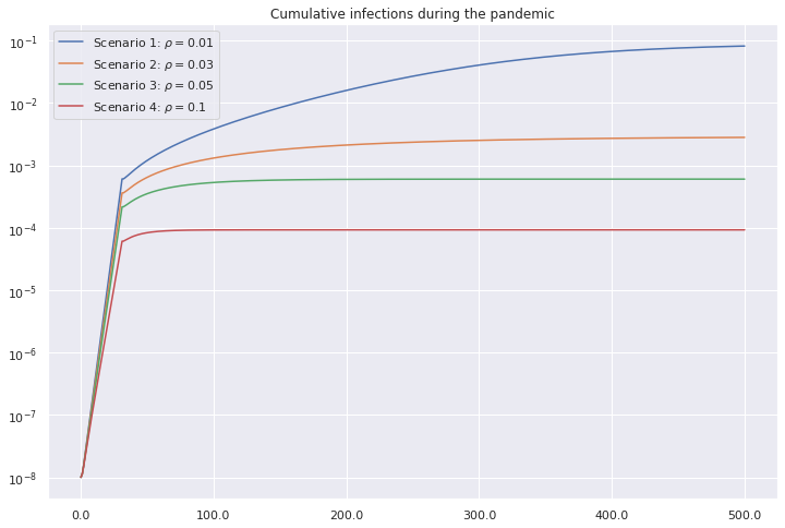
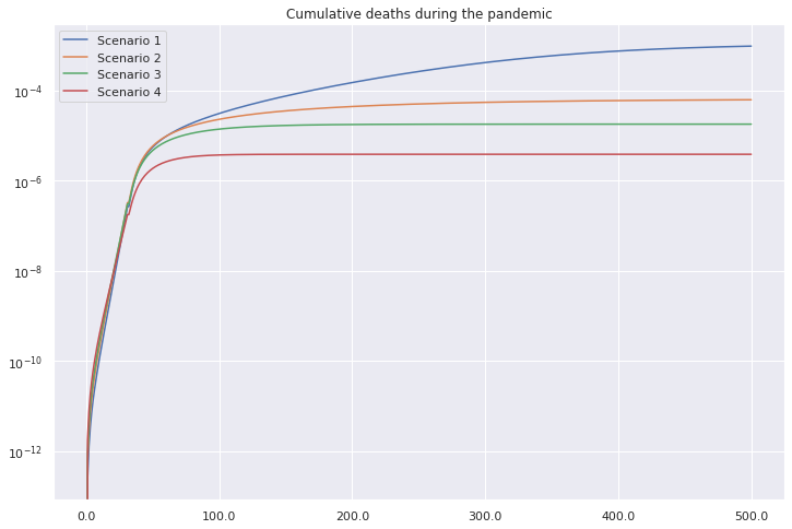
Also we have the testing rate \(\rho\) and it will vary from the values: \(0.01, 0.03, 0.05\) and \(0.1\).
It’s important to note the relation between the parameters \(\mu\) and \(\rho\). If \(\rho\) is high, we expect an increase of confirmed cases (compartment \(Q\)). If \(\mu\) is fixed, it will raise the deaths, as well. In this case, we note a relation between those parameters, not studied in the article.
However, when \(\rho\) parameter changes little, we expect \(\mu\) varies little too.
Using the Python script
- Open the file
parameters.yamland change the values as above: The parameterchange_pis reserved for the date when \(p\) changes. In this case, it will be \(31\). - Change the variable functions (\(r, \rho, \beta)\) in the class
Parameters_Functionsindynamics_model.pyfile. - Run
python execute_model.py. Follow the instructions to save the variables in the terminal.
The graphics were generated in the notebook graphics_website.ipynb.
The parameter \(\rho\) indicates the proportion of the population presenting either mild or no symptoms that is tested daily. It can also be thought as the inverse of the mean duration that an infected person in compartments A passes without being tested.
Another product of this work was the paper in the publications section:
Estimate of the rate of unreported COVID-19 cases during the first outbreak in Rio de Janeiro
In this work we fit an epidemiological model SEIAQR (Susceptible - Exposed - Infectious - Asymptomatic - Quarantined - Removed) to the data of the first COVID-19 outbreak in Rio de Janeiro, Brazil. Particular emphasis is given to the unreported rate, that is, the proportion of infected individuals that is not detected by the health system. The evaluation of the parameters of the model is based on a combination of error-weighted least squares method and appropriate B-splines. The structural and practical identifiability is analyzed to support the feasibility and robustness of the parameters’ estimation. We use the Bootstrap method to quantify the uncertainty of the estimates. For the outbreak of March–July 2020 in Rio de Janeiro, we estimate about 90% of unreported cases, with a 95% confidence interval (85%, 93%).